I am going to demonstrate a straightforward anomaly detection procedure using a limited toolset: SQLite.
Overview
Given the limited toolset, the algorithm must use nothing more than fundamental statistics (avg, variance, z-score) to identify atypical, anomalous events. We will be taking a step-by-step approach to build up the SQL query incrementally.
So, imagine you are monitoring some thing, taking multiple observations of various metrics. This could be:
- Account balances
- Heart rate and blood pressure of a patient
- CPU and memory utilization of a server
The goal is to identify when a anomaly, an outlier, an oddball occurs.
The dataset
This exact method imposes some requirements on the dataset. The dataset we’ll be using is stored in a SQLite table with the following columns:
tsgroup_namemetricvalue
ts is for timestamp, and it is expressed in unix time. That is, the
number of seconds since January 1, 1970. This allows for easy date
arithmetic and efficient date comparisons.
In this dataset, there are two groups and two metrics, with an
observation recorded in the events table every five minutes. There is
one row for each observation, so four rows for each observation period.
SELECT
  datetime(ts, 'unixepoch', 'localtime') as ts_local,
  ts,
  group_name,
  metric,
  value
FROM events
Top 8 rows:
| ts_local | ts | group_name | metric | value |
|---|---|---|---|---|
| 2018-12-22 06:00:00 | 1545458400 | Group A | Metric 1 | 222.24127 |
| 2018-12-22 06:00:00 | 1545458400 | Group B | Metric 1 | 252.97452 |
| 2018-12-22 06:00:00 | 1545458400 | Group A | Metric 2 | 34.57067 |
| 2018-12-22 06:00:00 | 1545458400 | Group B | Metric 2 | 38.94976 |
| 2018-12-22 06:05:00 | 1545458700 | Group A | Metric 1 | 253.60885 |
| 2018-12-22 06:05:00 | 1545458700 | Group B | Metric 1 | 200.50453 |
| 2018-12-22 06:05:00 | 1545458700 | Group A | Metric 2 | 32.67214 |
| 2018-12-22 06:05:00 | 1545458700 | Group B | Metric 2 | 35.75465 |
If you’d like, skip the explanation; get to the query.
Essential statistics
To compute the Z-score for each point, we will need the window average
and variance. We will build up to these stats using the window count
mov_n, window sum mov_sum, and window sum squared mov_sum_sq.
Since SQLite lacks functions for these window operations, they will
instead be calculated after performing a self-join of the table on the
ts column. Here you can define the window size, in seconds, by
subtracting a number of seconds from the timestamp of each point. Each
point then has a unique set of observations from which to calculate the
average and variance for. In this example, the window size is 10800
seconds, or 3 hours.
SELECT
  t1.ts,
  t1.group_name,
  t1.metric,
  t1.value,
  count(t2.value) AS mov_n,
  sum(t2.value) AS mov_sum,
  sum(t2.value*t2.value) AS mov_sum_sq
FROM events t1 LEFT JOIN events t2
  ON t1.group_name = t2.group_name
  AND t1.metric = t2.metric
  AND t2.ts >= t1.ts - 10800
  AND t2.ts < t1.ts
GROUP BY t1.ts,
  t1.group_name,
  t1.metric,
  t1.value
Top 12 rows:
| ts | group_name | metric | value | mov_n | mov_sum | mov_sum_sq |
|---|---|---|---|---|---|---|
| 1545458400 | Group A | Metric 1 | 222.24127 | 0 | NA | NA |
| 1545458400 | Group A | Metric 2 | 34.57067 | 0 | NA | NA |
| 1545458400 | Group B | Metric 1 | 252.97452 | 0 | NA | NA |
| 1545458400 | Group B | Metric 2 | 38.94976 | 0 | NA | NA |
| 1545458700 | Group A | Metric 1 | 253.60885 | 1 | 222.24127 | 49391.182 |
| 1545458700 | Group A | Metric 2 | 32.67214 | 1 | 34.57067 | 1195.131 |
| 1545458700 | Group B | Metric 1 | 200.50453 | 1 | 252.97452 | 63996.105 |
| 1545458700 | Group B | Metric 2 | 35.75465 | 1 | 38.94976 | 1517.083 |
| 1545459000 | Group A | Metric 1 | 231.62960 | 2 | 475.85012 | 113708.631 |
| 1545459000 | Group A | Metric 2 | 41.10389 | 2 | 67.24281 | 2262.600 |
| 1545459000 | Group B | Metric 1 | 225.97594 | 2 | 453.47904 | 104198.170 |
| 1545459000 | Group B | Metric 2 | 36.27989 | 2 | 74.70440 | 2795.478 |
Notice how the first few rows are missing some values. Also, mov_n,
the number of observations in the moving window, is 0. This is because
each observation computes the stats for a window of observations that
occured before it. Starting out, there are no past events to aggregate.
As we proceed, the window grows incrementally larger until a “complete”
window is obtained. See the last 12 observations:
| ts | group_name | metric | value | mov_n | mov_sum | mov_sum_sq |
|---|---|---|---|---|---|---|
| 1545543900 | Group A | Metric 1 | 247.15789 | 36 | 8354.390 | 1950818.35 |
| 1545543900 | Group A | Metric 2 | 28.81865 | 36 | 1236.088 | 42684.47 |
| 1545543900 | Group B | Metric 1 | 221.85380 | 36 | 8209.607 | 1880259.07 |
| 1545543900 | Group B | Metric 2 | 36.27406 | 36 | 1235.929 | 42750.46 |
| 1545544200 | Group A | Metric 1 | 211.70171 | 36 | 8367.339 | 1957051.38 |
| 1545544200 | Group A | Metric 2 | 37.93123 | 36 | 1230.194 | 42309.99 |
| 1545544200 | Group B | Metric 1 | 222.93765 | 36 | 8212.017 | 1881322.27 |
| 1545544200 | Group B | Metric 2 | 37.95745 | 36 | 1242.648 | 43192.78 |
| 1545544500 | Group A | Metric 1 | 224.19434 | 36 | 8362.074 | 1954794.53 |
| 1545544500 | Group A | Metric 2 | 36.77061 | 36 | 1234.598 | 42624.71 |
| 1545544500 | Group B | Metric 1 | 212.60191 | 36 | 8198.724 | 1875218.90 |
| 1545544500 | Group B | Metric 2 | 34.03929 | 36 | 1240.425 | 43019.12 |
With the building blocks for average and variance, we compute them and derive the Z-score for each point.
Average
What is typical.
$$ \bar{X}=\frac {\Sigma x} {N} $$
To SQL:
mov_sum/mov_n AS mov_avg
Variance
The query below uses the computational formula for variance.
$$ \sigma^2=\frac{ \Sigma{x^2}- \frac{ (\Sigma{x})^2 } N } {N-1} $$
To SQL:
( mov_sum_sq - (mov_sum*mov_sum)/mov_n ) / (mov_n - 1) AS mov_var
Z-score
From the stats above, we compute a Z-score. The Z-score is defined as number of standard deviations from the window average the current point is. In other words, it tells us how typical a new point is given past data. A threshold value is compared to the Z-score to classify points.
$$ z=\frac {x-\bar{X}} {\sigma} $$
This formula requires the standard deviation, σ, but we haven’t
computed that. We have the variance, σ2, so we take the
square root of variance to get the std. dev., right? Well, SQLite
doesn’t have a square root sqrt() function. Are we doomed? Somewhat,
but we will persevere. Sure, we could write a SQLite UDF, but let’s
instead keep this organic and work with what we’ve got. Square
everything to make use of the variance:
$$ z^2=\frac {(x-\bar{X})^2} {\sigma^2} $$
This is translated into SQL as:
((value - (mov_sum/mov_n)) * (value - (mov_sum/mov_n))) /   -- (value - mov_avg)^2 /
  ((mov_sum_sq - (mov_sum*mov_sum/mov_n)) / (mov_n - 1))    -- mov_var
Note that this is not the Z-score; this is the square of the Z-score.
So what do we do to get the real Z-score without a sqrt() function?
Beats me. But we don’t need the real Z-score; we can just square the
threshold to keep everything consistent.
Threshold
Again, a threshold is compared to the Z-score to decide whether a given point is an anomaly. This is the number of allowed standard deviations, and is a number of your choosing.
A threshold of 3 is a good starting point. Given this, a value is an
anomaly if mov_z_sq > 3*3.
That is:
$$ \frac {(x-\bar{X})^2} {\sigma^2}=z^2>\text{threshold}^2 $$
CASE
  WHEN
    ((value - (mov_sum/mov_n)) * (value - (mov_sum/mov_n))) /
    ((mov_sum_sq - (mov_sum*mov_sum/mov_n)) / (mov_n - 1)) > 3*3
    THEN 1
  ELSE 0
END is_anomaly
Remember to square the Z-score threshold.
The query
All together, the query starts by performing the non-equi self-join of
itself, the window size is 10800 seconds (3 hrs). From this, it
calculates the essential stats, the number of observerations mov_n,
moving sum mov_sum, moving sum2 mov_sum_sq. Built atop
that are statements that use these stats to return the moving average
mov_avg, moving variance mov_var, and moving z2
mov_z_sq. Finally, the threshold value 3 is squared and compared to
mov_z_sq to determine if the current point is atypical from previous
points in the moving window.
SELECT
 ts,
 group_name,
 metric,
 value,
 mov_n,
 mov_sum / mov_n AS mov_avg,
 (mov_sum_sq - (mov_sum*mov_sum/mov_n)) / (mov_n - 1) AS mov_var,
 ((value - (mov_sum/mov_n)) * (value - (mov_sum/mov_n))) / ((mov_sum_sq - (mov_sum*mov_sum/mov_n)) / (mov_n - 1)) AS mov_z_sq,
 CASE
    WHEN
     ((value - (mov_sum/mov_n)) * (value - (mov_sum/mov_n))) /
      ((mov_sum_sq - (mov_sum*mov_sum/mov_n)) / (mov_n - 1)) > 3*3 THEN 1
    ELSE 0
 END is_anomaly
FROM (
 SELECT
     t1.ts,
     t1.group_name,
     t1.metric,
     t1.value,
     count(t2.value) AS mov_n,
     sum(t2.value) AS mov_sum,
     sum(t2.value*t2.value) AS mov_sum_sq
 FROM events t1 LEFT JOIN events t2
  ON t1.group_name = t2.group_name
 AND t1.metric = t2.metric
 AND t2.ts >= t1.ts - 10800
 AND t2.ts < t1.ts
 GROUP BY t1.ts,
          t1.group_name,
          t1.metric,
          t1.value
) as t
Top 12 rows:
| ts | group_name | metric | value | mov_n | mov_avg | mov_var | mov_z_sq | is_anomaly |
|---|---|---|---|---|---|---|---|---|
| 1545543900 | Group A | Metric 1 | 247.15789 | 36 | 232.06639 | 344.148185 | 0.6617886 | 0 |
| 1545543900 | Group A | Metric 2 | 28.81865 | 36 | 34.33579 | 6.925934 | 4.3949084 | 0 |
| 1545543900 | Group B | Metric 1 | 221.85380 | 36 | 228.04465 | 231.485998 | 0.1655677 | 0 |
| 1545543900 | Group B | Metric 2 | 36.27406 | 36 | 34.33135 | 9.124584 | 0.4136195 | 0 |
| 1545544200 | Group A | Metric 1 | 211.70171 | 36 | 232.42607 | 350.391154 | 1.2257705 | 0 |
| 1545544200 | Group A | Metric 2 | 37.93123 | 36 | 34.17205 | 7.763974 | 1.8201274 | 0 |
| 1545544200 | Group B | Metric 1 | 222.93765 | 36 | 228.11157 | 230.463254 | 0.1161551 | 0 |
| 1545544200 | Group B | Metric 2 | 37.95745 | 36 | 34.51800 | 8.544728 | 1.3844604 | 0 |
| 1545544500 | Group A | Metric 1 | 224.19434 | 36 | 232.27983 | 355.812026 | 0.1837352 | 0 |
| 1545544500 | Group A | Metric 2 | 36.77061 | 36 | 34.29439 | 8.140444 | 0.7532325 | 0 |
| 1545544500 | Group B | Metric 1 | 212.60191 | 36 | 227.74235 | 229.204809 | 1.0001226 | 0 |
| 1545544500 | Group B | Metric 2 | 34.03929 | 36 | 34.45626 | 7.962866 | 0.0218349 | 0 |
View the results
Create a view of the query above to easily return anomalous records.
SELECT *
FROM v_anomaly
WHERE is_anomaly=1
| ts | group_name | metric | value | mov_n | mov_avg | mov_var | mov_z_sq | is_anomaly |
|---|---|---|---|---|---|---|---|---|
| 1545459000 | Group A | Metric 2 | 41.10389 | 2 | 33.62141 | 1.802205 | 31.06619 | 1 |
| 1545463500 | Group B | Metric 1 | 331.15989 | 17 | 226.16311 | 376.941435 | 29.24678 | 1 |
| 1545477900 | Group A | Metric 1 | 390.65061 | 36 | 229.25418 | 267.418941 | 97.40825 | 1 |
| 1545524700 | Group A | Metric 2 | 17.13078 | 36 | 34.06429 | 9.527033 | 30.09792 | 1 |
| 1545525300 | Group A | Metric 1 | 119.01052 | 36 | 229.91305 | 224.341019 | 54.82444 | 1 |
| 1545528600 | Group B | Metric 1 | 369.99453 | 36 | 229.41003 | 254.291812 | 77.72173 | 1 |
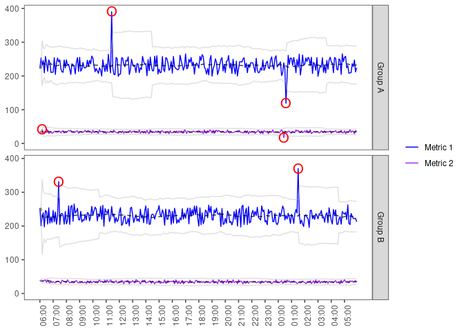
Visualized
Now that our original dataset is augmented with valuable statistics and
a classification, we can visualize the anomaly detection process. For
this, we will need to switch to R and import the packages RSQLite and
ggplot2. Also, since we’re now in R, we have a sqrt() function;
sweet. Note that, while R is among the best tools for analytics, the
anomaly detection process is being done entirely in SQL; we’re just
using R for the viz.
In the plot below, each group is plotted in a pane. Each group metric is plotted as a colored line. The window average is plotted as a black dashed line within each group metric. The light gray lines illustrate the define threshold which determines the classification. Notice how the threshold increases after an anomaly occurs, then drops back down after the window size (3 hrs) elapses.
library(RSQLite)
library(ggplot2)
library(data.table)

### Connect to and retrieve teh data

db <- dbConnect(RSQLite::SQLite(), db_name)

df_anom <- RSQLite::dbGetQuery(db, 'SELECT * FROM v_anomaly')

RSQLite::dbDisconnect(db)

### Quick prep

df_anom <- as.data.table(df_anom) # makes working with dataframes nicer.

df_anom[is.na(mov_avg), mov_avg := value]
df_anom[is.na(mov_var), mov_var := 0]

z_thresh <- 3 # define the threshold to visualize it. The classification has already been made.

df_anom[, ':=' (thresh_high = mov_avg + (sqrt(mov_var) * z_thresh),
                thresh_low = mov_avg - (sqrt(mov_var) * z_thresh),
                is_anomaly = as.logical(is_anomaly))]

### Visualize

ggplot(df_anom, aes(x=as.POSIXct(ts, origin='1970-01-01'), y=value)) +
        geom_line(aes(group=metric, color=metric)) +

        geom_line(aes(group=metric, y=mov_avg), color='black', alpha=0.8, linetype='dashed') +
        geom_line(aes(group=metric, y=thresh_high), color='gray', alpha=0.5) +
        geom_line(aes(group=metric, y=thresh_low), color='gray', alpha=0.5) +
        geom_point(data=df_anom[is_anomaly==TRUE,], color='red', shape='O', size=5) +

        facet_grid(rows=vars(group_name)) +
        scale_x_datetime(date_labels='%H:%M',
                        breaks=unique(df_anom[ts %% 3600 == 0,]$ts) %>% as.POSIXct(origin='1970-01-01')) +
        scale_colour_manual(values=c('blue', 'purple')) +
        labs(x=NULL, y=NULL) +
        theme_bw() +
        ylim(0, NA) +
        theme(axis.text.x = element_text(angle = 90),
              legend.title = element_blank(),
              panel.grid = element_blank())
Another Approach
The above approach implements a non-equi self-join on the ts column
with a window size defined in seconds. I felt this was the most
suitable way to describe this method of anomaly detection. However, a
faster query using windowing functions is shown below. Here, the window
size is not defined by time, but by the number of preceding points, so
it assumes periodic observations within the dataset. The clause
ROWS BETWEEN 36 PRECEDING AND 1 PRECEDING defines the window size to
be 35 preceding observations, not including the current observation. At
5 minute intervals, this equates to a window size of
35 point**s * 5 minutes * 60 seconds = 10500 seconds.
The query above has a window size of 10800 seconds, but the upper bound
is non-inclusive; the current point is not considered. We could have
made the upper bound <= 10500 seconds and achieve the same results.
Long story short, the query below will produce the same results as the
query above, but much faster, though with more assumptions and less
flexibility.
SELECT
  ts,
  group_name,
  metric,
  value,
  avg(value) OVER w as mov_avg,
  case
    when ((value - (avg(value) OVER w)) * (value - (avg(value) OVER w))) /
            (( (sum(value * value) OVER w) - ((sum(value) OVER w) * (avg(value) OVER w))) /
                ( (count(*) OVER w) - 1))
            > 3*3 THEN 1
    ELSE 0
  END as is_outlier
FROM events
WINDOW w AS (PARTITION BY group_name, metric ORDER BY ts ROWS BETWEEN 36 PRECEDING AND 1 PRECEDING)
ORDER by ts asc
Parting words
While the methods are fairly simple, this process will not detect outliers that occur within the defined threshold. Tools such as R and Python offer libraries that are better suited for more advanced anomaly detection tasks. However, I hope the approach described in this post serves to demystify the fundamental aspects of anomaly detection by using a simple toolset and elementary statistics.
Until next time,
Donald
